Key Takeaways
- Excel tables with structured references make your Gantt chart update automatically
- The WORKDAY.INTL function calculates end dates while excluding weekends
- Conditional formatting creates the visual timeline bars without manual drawing
Project management tools like Monday.com, Asana, and Microsoft Project cost anywhere from $10 to $55 per user per month. For small teams or one-off projects, that math doesn't work. Excel, which you probably already have, can build a Gantt chart that updates itself when you change task dates or durations.
The trick is combining Excel tables (which auto-expand and use structured references) with conditional formatting rules that draw the timeline bars for you. No VBA. No add-ins. Just formulas.
Step 1: Build the Data Table
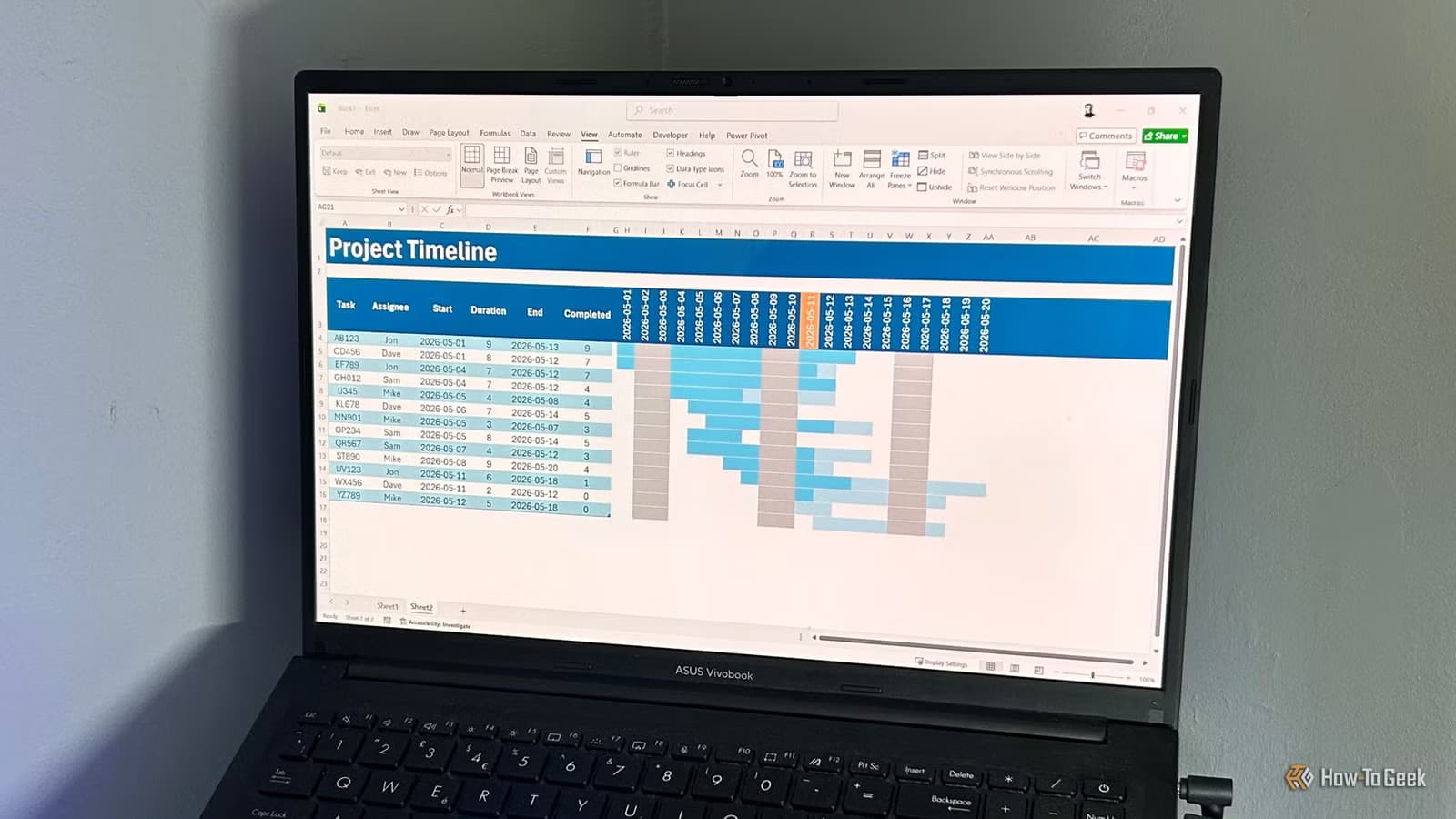
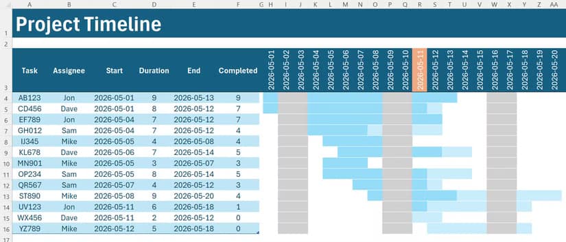
Start with a clean spreadsheet. In row 3, enter these column headers: Task, Assignee, Start, Duration, End, and Completed. Fill in your task IDs in the Task column.
Now convert this range into an Excel table. Select any cell in your data and press Ctrl+T. Check the box for "My table has headers" and click OK. This matters because Excel tables use structured references. When you add rows, formulas copy down automatically.
Rename the table to something memorable. Go to the Table Design tab and change the name to T_ProjectTimeline. While you're there, uncheck Filter Button to clean up the header row.
Step 2: Fill in the Columns
Each column serves a specific purpose:
- Assignee: Type names manually or use Data Validation to create a dropdown list
- Start: Format the column as a date (Ctrl+1, then choose Date), then enter your start dates
- Duration: Enter the number of days each task takes
- End: This gets calculated automatically
- Completed: Use a percentage or checkbox to track progress
Step 3: Calculate End Dates Automatically
The End column is where the automation starts. You have two options depending on whether your team works weekends.
For a simple calculation that includes weekends:
=[@Start]+[@Duration]For a calculation that excludes weekends, use the WORKDAY.INTL function:
=WORKDAY.INTL([@Start]-1,[@Duration])The -1 in the formula tells Excel to include the start date in the duration count. Without it, a task starting Monday with a 5-day duration would end on Monday instead of Friday.
Step 4: Add the Timeline Grid
To the right of your data table, create a date header row. Start with your project's first date and extend it across as many columns as your project spans. Use a formula like =A3+1 in each cell to auto-increment dates.
Format these cells to show just the day number or a short date format. This becomes the X-axis of your Gantt chart.
Step 5: Create the Bars with Conditional Formatting
This is where the visual magic happens. Select the entire grid area (all cells under your date headers, across all task rows). Then go to Home > Conditional Formatting > New Rule.
Choose "Use a formula to determine which cells to format." The formula checks whether each cell's column date falls between the task's start and end dates. When it does, the cell fills with color.
The basic logic: if the column header date is greater than or equal to the Start date AND less than or equal to the End date, apply a fill color.
Optional Enhancements
Once the basic chart works, you can add refinements:
- Weekend highlighting: Add a second conditional formatting rule that shades Saturday and Sunday columns gray
- Today marker: Use a rule that highlights the current date column with a vertical line
- Progress shading: If your Completed column tracks percentage, create a rule that fills bars partially based on completion
Why This Works Better Than You'd Expect
Excel tables use structured references like [@Start] instead of cell addresses like C4. When you add a new task row, every formula copies down automatically. When you change a start date or duration, the end date recalculates. The conditional formatting rules evaluate against the new values instantly.
The result is a Gantt chart that stays current without manual updates. Change a task's duration from 5 days to 8, and the bar extends. Push back a start date, and dependent visual elements shift.
Logicity's Take
More Microsoft Office productivity tricks
Another zero-cost productivity workaround
Frequently Asked Questions
Can I create a Gantt chart in Excel without macros?
Yes. Using Excel tables for your data and conditional formatting for the visual bars requires no VBA or macros. The chart updates automatically when you change task dates or durations.
How do I exclude weekends from Excel Gantt chart calculations?
Use the WORKDAY.INTL function instead of simple addition. The formula =WORKDAY.INTL([@Start]-1,[@Duration]) calculates end dates while skipping Saturdays and Sundays.
What's the advantage of using Excel tables for a Gantt chart?
Excel tables use structured references that automatically extend to new rows. When you add a task, all formulas copy down without manual intervention.
Can I show task progress in an Excel Gantt chart?
Yes. Add a Completed percentage column, then create an additional conditional formatting rule that partially fills task bars based on that percentage value.
Need Help Implementing This?
Source: How-To Geek
Manaal Khan
Tech & Innovation Writer
Produced with AI assistance and reviewed by the Logicity editorial team. Learn more in our Editorial Policy.