Excel Dynamic Arrays: One Formula, Thousands of Results
Key Takeaways
- Dynamic arrays allow one formula to output multiple results that automatically expand or contract
- The FILTER, SORTBY, UNIQUE, and XLOOKUP functions can replace thousands of legacy formulas
- Dynamic arrays don't work inside Excel tables. Place them outside the table grid with empty cells nearby
If you're still dragging formulas down thousands of rows or copying and pasting data between sheets, Excel's dynamic array functions are about to save you hours. These functions let a single formula return an entire block of results that automatically grows or shrinks as your source data changes.
"Dynamic arrays are the most significant change to the Excel calculation engine in over 30 years," said Joe McDaid, Program Manager for Excel, when Microsoft first announced the feature. That's not marketing hype. The calculation engine itself was rebuilt to support this behavior.
What Changed: From One Cell to Many
Traditional Excel formulas follow a simple rule: one formula, one cell, one result. Want to apply a calculation to 1,000 rows? You need to copy that formula 1,000 times. Add more data? Copy the formula again.
Dynamic arrays break this pattern. Type a formula in one cell, press Enter, and the results "spill" into neighboring cells. A thin blue border marks the spill range. Add rows to your source data, and the spill range expands automatically. Delete rows, and it contracts.
This replaces the old Ctrl+Shift+Enter (CSE) array formulas that experienced Excel users learned to fear. CSE formulas were powerful but notoriously difficult to build, edit, and debug. Dynamic arrays deliver the same power with standard formula entry.
Where Dynamic Arrays Work
Dynamic array functions are available in Microsoft 365, Excel 2021, Excel 2024, and Excel for the web. If you're running an older version, these formulas won't work.
There's one critical limitation: dynamic arrays can't spill inside Excel tables. The structured reference system that tables use conflicts with spill behavior. Place your dynamic array formulas outside the table grid, and leave at least one empty column or row for the results to expand into.
The Core Functions You Need
Microsoft started with 6 dynamic array functions and has since expanded to over 50. Here are the ones that handle most real-world scenarios.
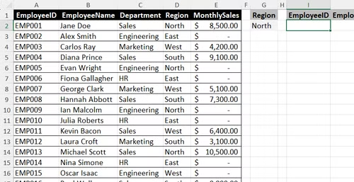
FILTER: Extract Rows That Match Criteria
FILTER returns all rows from a dataset where a condition is true. Need all sales records from the West region? One formula: =FILTER(A2:D100, B2:B100="West"). The result spills into as many rows as match your criteria.
You can combine conditions with multiplication (AND logic) or addition (OR logic). To filter for West region AND sales over $10,000: =FILTER(A2:D100, (B2:B100="West")*(C2:C100>10000)).
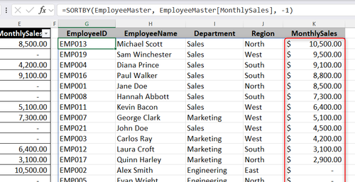
SORTBY: Arrange Data by Any Column
SORTBY returns a sorted copy of your data without altering the original. Unlike the SORT function, SORTBY lets you sort by a column that isn't included in your output.
To sort a dataset by monthly sales in descending order: =SORTBY(A2:D100, D2:D100, -1). The -1 indicates descending order. Use 1 for ascending.
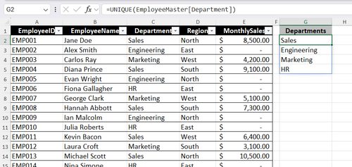
UNIQUE: Extract Distinct Values
UNIQUE pulls a list of distinct values from a column. If your employee records contain 500 rows with 8 different departments, =UNIQUE(C2:C500) returns just those 8 department names.
This function also has an optional parameter to return values that appear only once. Set the second argument to TRUE: =UNIQUE(C2:C500, FALSE, TRUE).
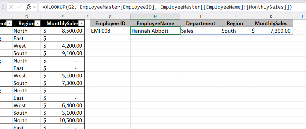
XLOOKUP: The Better VLOOKUP
XLOOKUP replaces VLOOKUP, HLOOKUP, and INDEX/MATCH combinations. It searches left or right, handles errors gracefully, and can return multiple columns at once.
To find an employee by ID and return their name, department, and salary: =XLOOKUP(G2, A2:A100, B2:D100). The result spills across three columns.
The #SPILL! Error and How to Fix It
The most common frustration with dynamic arrays is the #SPILL! error. It appears when the spill range is blocked by existing data. Excel won't overwrite cells that contain values, even spaces or empty strings.
To fix it: click the error indicator and select "Select Obstructing Cells." Excel highlights the cells blocking your formula. Clear them, and the formula spills normally.
Reddit's r/excel community has developed a design philosophy around preventing #SPILL! errors. Users call it "5G Modeling," which emphasizes leaving clean buffer zones around spill ranges and avoiding merged cells entirely.
“It makes you feel like an 'evil wizard' because of how much power a single cell suddenly holds.”
— Anonymous user, Reddit r/excel community
Combining Functions for Complex Workflows
The real power emerges when you nest these functions. Want a sorted, filtered list of unique values? Chain them together.
Example: extract all West region employees, sort by salary descending, return unique departments: =UNIQUE(SORTBY(FILTER(A2:D100, B2:B100="West"), D2:D100, -1)).
Each function processes the output of the one inside it. The FILTER runs first, SORTBY orders the filtered results, and UNIQUE extracts distinct values from that sorted list.
When to Use Dynamic Arrays vs. Power Query
Dynamic arrays work best for medium-sized datasets where you need live, formula-based results. If your data changes frequently and you want outputs that update instantly, dynamic arrays are the right choice.
For larger datasets, external data sources, or complex transformations that involve multiple steps, Power Query is usually better. Power Query handles millions of rows and provides a visual interface for building transformation pipelines.
- Use dynamic arrays for: live dashboards, lookup tables, filtered views of internal data
- Use Power Query for: importing external files, combining multiple sources, data cleaning at scale
Logicity's Take
Frequently Asked Questions
Do dynamic arrays work in Google Sheets?
Google Sheets has supported array formulas for years, but the syntax differs. Functions like FILTER and UNIQUE exist in both, though Google Sheets uses ARRAYFORMULA for some behaviors that Excel handles automatically.
Why does my dynamic array formula show #SPILL!?
The spill range is blocked by existing data. Click the error indicator, select 'Select Obstructing Cells,' and clear those cells. Even invisible characters like spaces can block the spill.
Can I use dynamic arrays inside Excel tables?
No. Dynamic arrays can't spill inside structured tables. Place your formula outside the table and reference the table data from there.
What Excel versions support dynamic arrays?
Microsoft 365, Excel 2021, Excel 2024, and Excel for the web. Earlier versions like Excel 2019 and 2016 don't support dynamic array behavior.
How do I reference a spill range in another formula?
Use the spill range operator: add # after the cell containing your dynamic array formula. If your formula is in A1, reference the entire spill range as A1#.
Another technical workaround for common infrastructure limitations
Need Help Implementing This?
Source: How-To Geek
Huma Shazia
Senior AI & Tech Writer
اقرأ أيضاً

رأي مغاير: كيف يؤثر اختراق الأمن الداخلي الأميركي على شركاتنا الخاصة؟
في ظل اختراق عقود الأمن الداخلي الأميركي مع شركات خاصة، نناقش تأثير هذا الاختراق على مستقبل الأمن السيبراني. نستعرض الإحصاءات الموثوقة ونناقش كيف يمكن للشركات الخاصة أن تتعامل مع هذا التهديد. استمتع بقراءة هذا التحليل العميق

الإنسان في زمن ما بعد الوجود البشري: نحو نظام للتعايش بين الإنسان والروبوت - Centre for Arab Unity Studies
في هذا المقال، سنناقش كيف يمكن للبشر والروبوتات التعايش في نظام متكامل. سنستعرض التحديات والحلول المحتملة التي تضعها شركات مثل جوجل وأمازون. كما سنلقي نظرة على التوقعات المستقبلية وفقًا لتقرير ماكنزي

إطلاق ناسا لمهمة مأهولة إلى القمر: خطوة تاريخية نحو استكشاف الفضاء
تعتبر المهمة الجديدة خطوة هامة نحو استكشاف الفضاء وتطوير التكنولوجيا. سوف تشمل المهمة إرسال رواد فضاء إلى سطح القمر لconducting تجارب علمية. ستسهم هذه المهمة في تطوير فهمنا للفضاء وتحسين التكنولوجيا المستخدمة في استكشاف الفضاء.