Excel Conditional Formatting: 5 Rules That Fix Ugly Spreadsheets

Key Takeaways
- Conditional formatting applies colors and icons based on rules, not manual selection
- Built-in presets like color scales work instantly without formulas
- Using Excel Tables (Ctrl+T) makes formatting rules extend automatically to new rows
The Problem With Most Spreadsheets
Open any spreadsheet built by someone who learned Excel last week. You'll see the same thing: rows and columns of identical, unstyled numbers that require effort to interpret. The data might be accurate. The problem is the lack of visual structure.
Without visual cues, your brain has to manually sort out what matters. Trends, outliers, and errors sit buried in a uniform grid. You can manually add colors or borders to fix this, but that approach breaks the moment values change. Your formatting becomes outdated or inconsistent.
Conditional formatting solves this by making formatting rule-based instead of manual. Set up a rule once, and Excel applies and updates the styling automatically as your data changes.
1. Use Excel Tables First
Before applying any conditional formatting, convert your data range to an Excel Table. Select your data and press Ctrl+T (or Cmd+T on Mac). This step matters because conditional formatting rules applied to Tables automatically extend to new rows as you add data.
Skip this step and you'll find yourself re-applying rules every time your dataset grows. Tables keep everything dynamic.
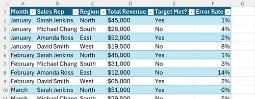
2. Apply Color Scales for Instant Heat Maps
The fastest way to improve readability is letting Excel apply structure for you. Color scales convert raw numbers into visual patterns without requiring formulas.
Select a column of numbers. Go to Home > Conditional Formatting > Color Scales. Pick a two-color or three-color gradient. Excel automatically assigns colors based on each cell's value relative to the range. High values get one color, low values get another, and middle values blend between them.
This works well for revenue figures, inventory counts, or any numeric column where spotting highs and lows quickly matters. A massive inventory spreadsheet with hundreds of rows becomes scannable in seconds.
3. Add Icon Sets for Status Indicators
Icon sets place small graphics (arrows, traffic lights, flags) inside cells based on value thresholds. They're useful for columns that represent performance or status.
Select your data, go to Home > Conditional Formatting > Icon Sets, and choose a style. Excel divides your range into thirds by default and assigns icons accordingly. Green arrows or checkmarks go to the top third, yellow to the middle, red to the bottom.
You can customize the thresholds if the default splits don't match your criteria. Click Manage Rules, edit the rule, and set specific values or percentages for each icon tier.
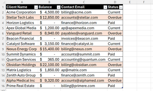
4. Highlight Cells That Meet Specific Conditions
Beyond gradients and icons, conditional formatting can highlight cells based on specific criteria. Want to flag every value above 10,000? Every cell containing the word 'Overdue'? Every date in the past?
Go to Home > Conditional Formatting > Highlight Cells Rules. Options include Greater Than, Less Than, Between, Equal To, Text That Contains, and Date Occurring. Select your condition, set the threshold, and pick a fill color.
This approach is more targeted than color scales. Instead of showing relative value across a range, it flags specific items that need attention.
5. Format Entire Rows Based on One Column
The previous rules format individual cells. Sometimes you need to highlight an entire row when one column meets a condition. A client dashboard might need all rows with 'Overdue' status to appear in red, not just the status cell.
This requires a formula-based rule. Select your entire data range (all columns, all rows). Go to Home > Conditional Formatting > New Rule > Use a formula to determine which cells to format.
Enter a formula that references the column you want to check. If your status column is column E and your data starts in row 2, the formula might be =$E2="Overdue". The dollar sign before E locks the column reference while allowing the row number to change. Set your fill color and apply.
Now every row where column E contains 'Overdue' gets highlighted across all columns.
Managing and Editing Rules
Rules stack. If you apply multiple conditional formats to the same range, they're evaluated in order. Go to Home > Conditional Formatting > Manage Rules to see all rules for your current selection or the entire sheet.
From this dialog, you can edit rule criteria, change formatting, adjust the order of evaluation, or delete rules that no longer apply. If two rules conflict, the one higher in the list takes precedence.
Logicity's Take
Frequently Asked Questions
Does conditional formatting slow down large spreadsheets?
It can if you apply complex formula-based rules to thousands of rows. Built-in presets like color scales have minimal performance impact. If you notice slowdown, consolidate rules or limit their range.
Can I copy conditional formatting to another sheet?
Yes. Select a cell with the formatting you want, press Ctrl+C, then select the target range and use Paste Special > Formatting (or just the paintbrush Format Painter tool).
Why doesn't my conditional formatting update when data changes?
Check that your rule's 'Applies to' range covers all your data. If you didn't use an Excel Table, the range might not include new rows. Edit the rule and expand the range, or convert to a Table.
Can I use conditional formatting with text, not just numbers?
Yes. The 'Text That Contains' rule highlights cells with specific words or phrases. Formula-based rules can check text length, starting characters, or other string conditions.
If you're looking for Excel alternatives with similar formatting features
Need Help Implementing This?
Source: How-To Geek
Manaal Khan
Tech & Innovation Writer
اقرأ أيضاً

رأي مغاير: كيف يؤثر اختراق الأمن الداخلي الأميركي على شركاتنا الخاصة؟
في ظل اختراق عقود الأمن الداخلي الأميركي مع شركات خاصة، نناقش تأثير هذا الاختراق على مستقبل الأمن السيبراني. نستعرض الإحصاءات الموثوقة ونناقش كيف يمكن للشركات الخاصة أن تتعامل مع هذا التهديد. استمتع بقراءة هذا التحليل العميق

الإنسان في زمن ما بعد الوجود البشري: نحو نظام للتعايش بين الإنسان والروبوت - Centre for Arab Unity Studies
في هذا المقال، سنناقش كيف يمكن للبشر والروبوتات التعايش في نظام متكامل. سنستعرض التحديات والحلول المحتملة التي تضعها شركات مثل جوجل وأمازون. كما سنلقي نظرة على التوقعات المستقبلية وفقًا لتقرير ماكنزي

إطلاق ناسا لمهمة مأهولة إلى القمر: خطوة تاريخية نحو استكشاف الفضاء
تعتبر المهمة الجديدة خطوة هامة نحو استكشاف الفضاء وتطوير التكنولوجيا. سوف تشمل المهمة إرسال رواد فضاء إلى سطح القمر لconducting تجارب علمية. ستسهم هذه المهمة في تطوير فهمنا للفضاء وتحسين التكنولوجيا المستخدمة في استكشاف الفضاء.